44 multiple data labels excel pie chart
› pie-chart-examplesPie Chart Examples | Types of Pie Charts in Excel with Examples PIE Chart can be defined as a circular chart with multiple divisions in it, and each division represents some portion of a total circle or total value. Simply each circle represents the total value of 100 per cent, and each division contributes some per cent to the total. Create A Pie Chart From Excel Data - PieProNation.com How To Create A Pie Chart. Just like any chart, we can easily create a pie chart in Excel version 2013, 2010 or lower. First, we select the data we want to graph. Click Insert tab, Pie button then choose from the selection of pie chart types: Pie, Exploded Pie, Pie of pie, Bar of pie, or 3D pie chart. Figure 2.
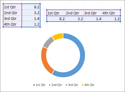
Doughnut Chart in Excel | How to Create Doughnut Excel Chart? Doughnut Chart is a part of a Pie chart in excel Pie Chart In Excel Making a pie chart in excel can help you with the pictorial representation of your data and simplifies the analysis process. There are multiple kinds of pie chart options available on excel to serve the varying user needs. read more. A pie occupies the entire chart, but it will ...

Multiple data labels excel pie chart
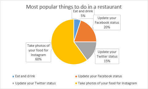
How to Show Percentage in Pie Chart in Excel? - GeeksforGeeks 29/06/2021 · Select a 2-D pie chart from the drop-down. A pie chart will be built. Select -> Insert -> Doughnut or Pie Chart -> 2-D Pie. Initially, the pie chart will not have any data labels in it. To add data labels, select the chart and then click on the “+” button in the top right corner of the pie chart and check the Data Labels button. Pie Chart in Excel - Inserting, Formatting, Filters, Data Labels Click on the Instagram slice of the pie chart to select the instagram. Go to format tab. (optional step) In the Current Selection group, choose data series "hours". This will select all the slices of pie chart. Click on Format Selection Button. As a result, the Format Data Point pane opens. How to Make a Pie Chart in Excel: 10 Steps (with Pictures) - wikiHow 18/04/2022 · Click the "Pie Chart" icon. This is a circular button in the "Charts" group of options, which is below and to the right of the Insert tab. You'll see several options appear in a drop-down menu: 2-D Pie - Create a simple pie chart that displays color-coded sections of your data. 3-D Pie - Uses a three-dimensional pie chart that displays color ...
Multiple data labels excel pie chart. Pie Chart Examples | Types of Pie Charts in Excel with Examples PIE Chart can be defined as a circular chart with multiple divisions in it, and each division represents some portion of a total circle or total value. ... Right-click and choose the “Add Data Labels “option for additional drop-down options. From that drop-down, select the option “Add Data Callouts”. ... Here we discuss Types of Pie ... Multiple pie charts in excel - MorvenNihal You can find many examples of templates and learn to structure your. In the Insert tab from the Charts section select the Insert Pie or Doughnut Chart option its shaped like a tiny pie chart. If a row has a digit of. Click on the Pie Chart click the icon checktick the Data Labels checkbox in the Chart Element box select. How to quickly create bubble chart in Excel? - ExtendOffice 5. if you want to add label to each bubble, right click at one bubble, and click Add Data Labels > Add Data Labels or Add Data Callouts as you need. Then edit the labels as you need. If you want to create a 3-D bubble chart, after creating the basic bubble chart, click Insert > Scatter (X, Y) or Bubble Chart > 3-D Bubble. How to ☝️ Create a Chart with Three Variables in Excel 14/07/2022 · How to Graph Three Variables in Excel. 1. Select your data. 2. Navigate to the Insert tab.. 3. In the Chart section, choose Insert Column or Bar Chart.. 4. Pick the chart style you like. Easy-peasy! Just like that, you have produced a graph with three variables in a matter of seconds.
How to Add Axis Labels in Excel Charts - Step-by-Step (2022) How to Add Axis Labels in Excel Charts – Step-by-Step (2022) An axis label briefly explains the meaning of the chart axis. It’s basically a title for the axis. Like most things in Excel, it’s super easy to add axis labels, when you know how. So, let me show you 💡. If you want to tag along, download my sample data workbook here. › how-to-show-percentage-inHow to Show Percentage in Pie Chart in Excel? - GeeksforGeeks Jun 29, 2021 · Select a 2-D pie chart from the drop-down. A pie chart will be built. Select -> Insert -> Doughnut or Pie Chart -> 2-D Pie. Initially, the pie chart will not have any data labels in it. To add data labels, select the chart and then click on the “+” button in the top right corner of the pie chart and check the Data Labels button. How to create a chart in Excel from multiple sheets - Ablebits.com 29/09/2022 · Supposing you have a few worksheets with revenue data for different years and you want to make a chart based on those data to visualize the general trend. 1. Create a chart based on your first sheet. Open your first Excel worksheet, select the data you want to plot in the chart, go to the Insert tab > Charts group, and choose the chart type you ... How to Create a Dynamic Pie Chart in Excel? - GeeksforGeeks It is the easiest method for creating a dynamic pie chart. So to this follow the following steps: Step 1: Create a table with proper headings and values inserted in it. Here, a table is created with Year-wise Sale, Tax, and Total (Sum of Sale and Tax) columns. Step 2: Copy the headings and paste them separately.
Pie of Pie Chart in Excel - Inserting, Customizing - Excel Unlocked Inserting a Pie of Pie Chart. Let us say we have the sales of different items of a bakery. Below is the data:-. To insert a Pie of Pie chart:-. Select the data range A1:B7. Enter in the Insert Tab. Select the Pie button, in the charts group. Select Pie of Pie chart in the 2D chart section. Excel Pie Chart Multiple Data Labels - Multiplication Chart Printable Excel Pie Chart Multiple Data Labels - You can create a multiplication chart in Stand out simply by using a template. You will find a number of samples of themes and learn how to file format your multiplication graph or chart using them. Below are a few tips and tricks to make a multiplication chart. › how-to-create-excel-pie-chartsHow to Make a Pie Chart in Excel & Add Rich Data Labels to ... Sep 08, 2022 · In this article, we are going to see a detailed description of how to make a pie chart in excel. One can easily create a pie chart and add rich data labels, to one’s pie chart in Excel. So, let’s see how to effectively use a pie chart and add rich data labels to your chart, in order to present data, using a simple tennis related example. › office-addins-blog › create-chartHow to create a chart in Excel from multiple sheets Sep 29, 2022 · Supposing you have a few worksheets with revenue data for different years and you want to make a chart based on those data to visualize the general trend. 1. Create a chart based on your first sheet. Open your first Excel worksheet, select the data you want to plot in the chart, go to the Insert tab > Charts group, and choose the chart type you ...
How To Make Pie Chart With Column Chart Detail - danryan.us
› Make-a-Pie-Chart-in-ExcelHow to Make a Pie Chart in Excel: 10 Steps (with Pictures) Apr 18, 2022 · Click the "Pie Chart" icon. This is a circular button in the "Charts" group of options, which is below and to the right of the Insert tab. You'll see several options appear in a drop-down menu: 2-D Pie - Create a simple pie chart that displays color-coded sections of your data. 3-D Pie - Uses a three-dimensional pie chart that displays color ...
How to Make a Pie Chart with Multiple Data in Excel (2 Ways)
EOF

Best Excel Tutorial - Multi Level Pie Chart
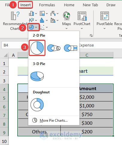
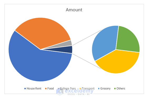
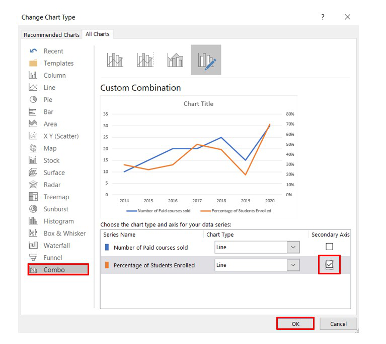
How to Make a Pie Chart with Multiple Data in Excel (2 Ways) - ExcelDemy Steps: First, select the entire data set and go to the Insert tab from the ribbon. After that, choose Insert Pie and Doughnut Chart from the Charts group. Afterward, click on the 2nd Pie Chart among the 2-D Pie as marked on the following picture. Now, Excel will instantly create a Pie of Pie Chart in your worksheet.

How to Create a Pie Chart in Excel | Smartsheet
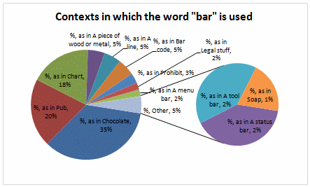
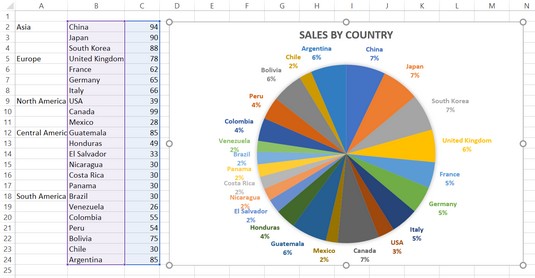
Excel Prevent overlapping of data labels in pie chart I have a lot of dynamic pie charts in excel. I must use a pie chart, but my data labels (percentage, value, name) overlapping. How can I fix it except the best-fit option? My two cents, maybe not the answer you're expecting, but don't use a pie chart for this. Too many slices in a pie chart makes the chart unreadable.
How to Make a Pie Chart with Multiple Data in Excel (2 Ways)
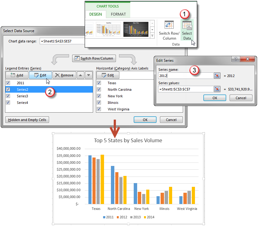
Select data for a chart - support.microsoft.com For this chart. Arrange the data. Column, bar, line, area, surface, or radar chart. Learn more abut. column, bar, line, area, surface, and radar charts. In columns or rows. Pie chart. This chart uses one set of values (called a data series). Learn more about. pie charts. In one column or row, and one column or row of labels. Doughnut chart

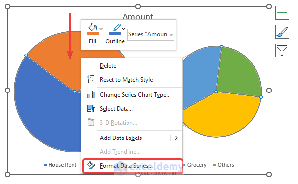
Creating Pie Chart and Adding/Formatting Data Labels (Excel)
excel - How to not display labels in pie chart that are 0% - Stack Overflow Generate a new column with the following formula: =IF (B2=0,"",A2) Then right click on the labels and choose "Format Data Labels". Check "Value From Cells", choosing the column with the formula and percentage of the Label Options. Under Label Options -> Number -> Category, choose "Custom". Under Format Code, enter the following:
How to Create a Graph with Multiple Lines in Excel | Pryor ...
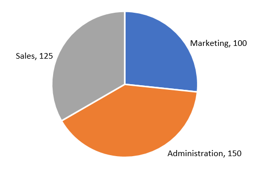
Excel Pie Chart Labels on Slices: Add, Show & Modify Factors - ExcelDemy The method to add category names to the data labels is given below step-by-step: 📌 Steps: First, double-click on the data labels on the pie chart. As a result, a side window called Format Data Labels will appear. Now, go to the drop-down of the Label Options to Label Options tab. Then, check the Category Name option.
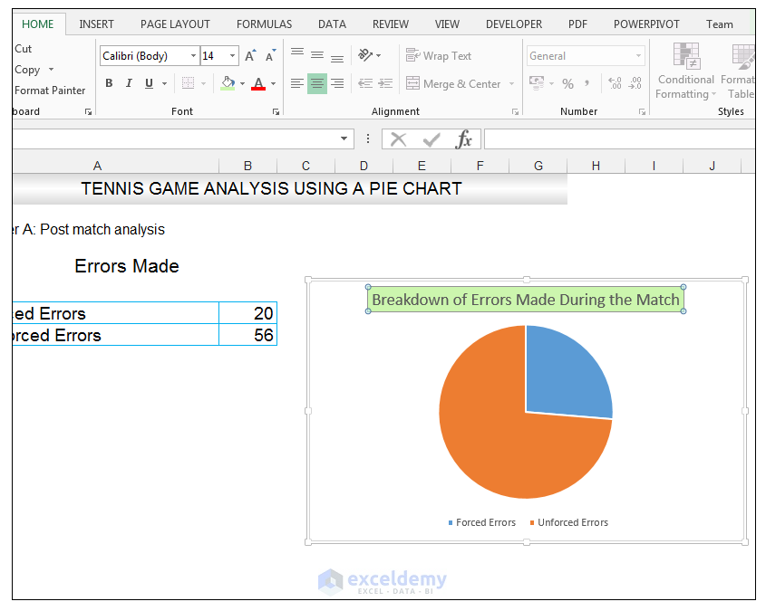
How to Make a Pie Chart in Excel & Add Rich Data Labels to ...
How To Add Multiple Data Labels In Excel Chart Here are several tips and tricks to generate a multiplication graph. Once you have a format, all you need to do is backup the solution and paste it in a new cell. After that you can take advantage of this formula to multiply a series of numbers by an additional established. How To Add Multiple Data Labels In Excel Chart. Multiplication desk ...
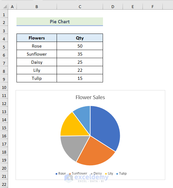
How to Create a Pie Chart in Excel using Worksheet Data
support.microsoft.com › en-us › officeSelect data for a chart - support.microsoft.com For this chart. Arrange the data. Column, bar, line, area, surface, or radar chart. Learn more abut. column, bar, line, area, surface, and radar charts. In columns or rows. Pie chart. This chart uses one set of values (called a data series). Learn more about. pie charts. In one column or row, and one column or row of labels. Doughnut chart
How to Make a Pie Chart with Multiple Data in Excel (2 Ways)
How to Make a Pie Chart in Excel & Add Rich Data Labels to The Chart! 08/09/2022 · A pie chart is used to showcase parts of a whole or the proportions of a whole. There should be about five pieces in a pie chart if there are too many slices, then it’s best to use another type of chart or a pie of pie chart in order to showcase the data better. In this article, we are going to see a detailed description of how to make a pie chart in excel.

Add or remove data labels in a chart
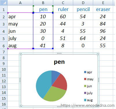
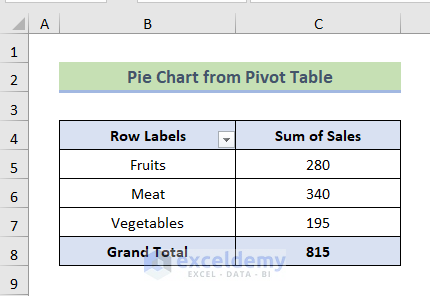
› documents › excelHow to show percentage in pie chart in Excel? - ExtendOffice 1. Select the data you will create a pie chart based on, click Insert > Insert Pie or Doughnut Chart > Pie. See screenshot: 2. Then a pie chart is created. Right click the pie chart and select Add Data Labels from the context menu. 3. Now the corresponding values are displayed in the pie slices. Right click the pie chart again and select Format ...

How to make a pie chart in Excel
How to Make a Pie Chart in Excel: 10 Steps (with Pictures) - wikiHow 18/04/2022 · Click the "Pie Chart" icon. This is a circular button in the "Charts" group of options, which is below and to the right of the Insert tab. You'll see several options appear in a drop-down menu: 2-D Pie - Create a simple pie chart that displays color-coded sections of your data. 3-D Pie - Uses a three-dimensional pie chart that displays color ...
Automatically Group Smaller Slices in Pie Charts to one big Slice
Pie Chart in Excel - Inserting, Formatting, Filters, Data Labels Click on the Instagram slice of the pie chart to select the instagram. Go to format tab. (optional step) In the Current Selection group, choose data series "hours". This will select all the slices of pie chart. Click on Format Selection Button. As a result, the Format Data Point pane opens.

How to Show Percentage in Pie Chart in Excel? - GeeksforGeeks
How to Show Percentage in Pie Chart in Excel? - GeeksforGeeks 29/06/2021 · Select a 2-D pie chart from the drop-down. A pie chart will be built. Select -> Insert -> Doughnut or Pie Chart -> 2-D Pie. Initially, the pie chart will not have any data labels in it. To add data labels, select the chart and then click on the “+” button in the top right corner of the pie chart and check the Data Labels button.
How to Make a Pie Chart with Multiple Data in Excel (2 Ways)

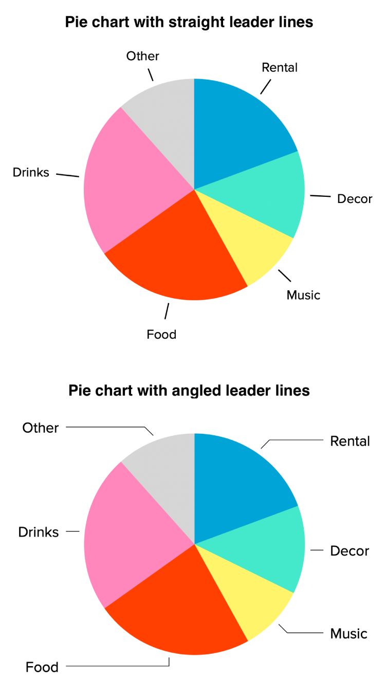
How to Make Pie Chart with Labels both Inside and Outside ...
Rotate charts in Excel - spin bar, column, pie and line charts
How to Create a Graph with Multiple Lines in Excel | Pryor ...

How to Data Labels in a Pie chart in Excel 2010
5 New Charts to Visually Display Data in Excel 2019 - dummies
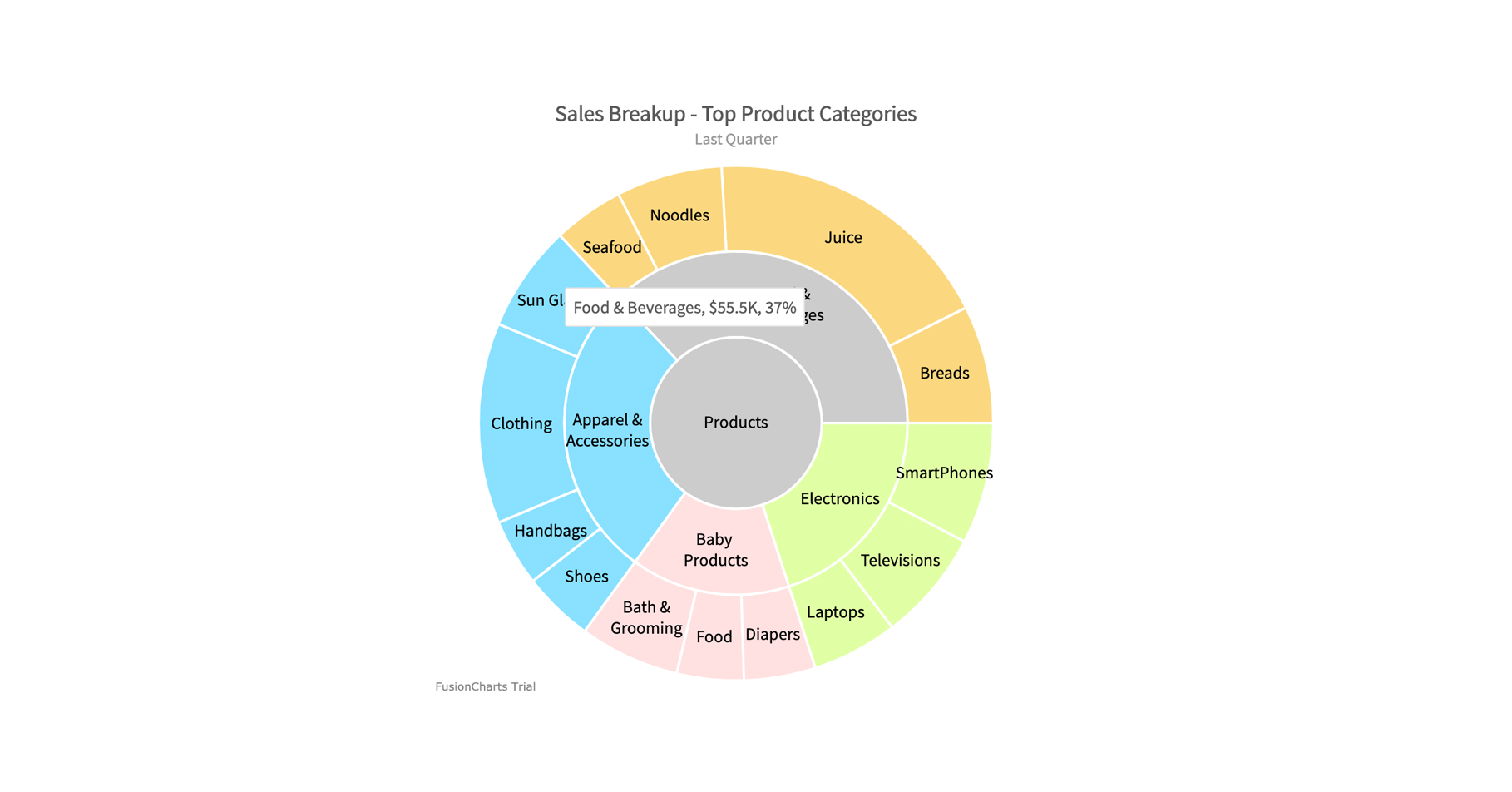
Multi-level Pie Chart | FusionCharts

Add or remove data labels in a chart

excel - Finding multiple local maxima and placing data labels ...

Custom data labels in a chart

Optimally positioning pie chart data labels in Excel with VBA ...
![How to Make a Chart or Graph in Excel [With Video Tutorial]](https://blog.hubspot.com/hs-fs/hubfs/Google%20Drive%20Integration/How%20to%20Make%20a%20Chart%20or%20Graph%20in%20Excel%20%5BWith%20Video%20Tutorial%5D-Aug-05-2022-05-11-54-88-PM.png?width=624&height=780&name=How%20to%20Make%20a%20Chart%20or%20Graph%20in%20Excel%20%5BWith%20Video%20Tutorial%5D-Aug-05-2022-05-11-54-88-PM.png)
How to Make a Chart or Graph in Excel [With Video Tutorial]
How to make a multilayer pie chart in Excel
Select data for a chart

How to make a Pie Chart in Excel

EXCEL Charts: Column, Bar, Pie and Line

How to Show Percentage in Pie Chart in Excel? - GeeksforGeeks

Change color of data label placed, using the 'best fit ...
Change the look of chart text and labels in Numbers on Mac ...

Plot Multiple Data Sets on the Same Chart in Excel ...
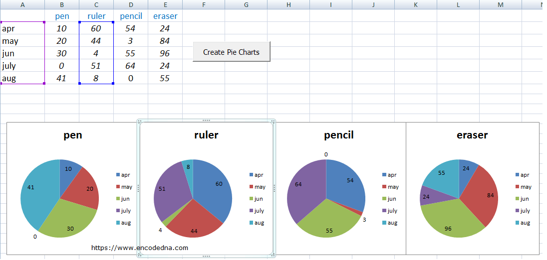
Create Multiple Pie Charts in Excel using Worksheet Data and VBA

Power BI Pie Chart - Complete Tutorial - SPGuides
Plot Multiple Data Sets on the Same Chart in Excel ...
How to fix wrapped data labels in a pie chart | Sage Intelligence

How to show data labels in PowerPoint and place them ...
How to Make Pie Chart with Labels both Inside and Outside ...
How to Make a Pie Chart with Multiple Data in Excel (2 Ways)

Automatically Group Smaller Slices in Pie Charts to one big Slice

Microsoft Excel Tutorials: Add Data Labels to a Pie Chart

How to create pie of pie or bar of pie chart in Excel?
Post a Comment for "44 multiple data labels excel pie chart"