44 excel chart hide zero data labels

› charts › dynamic-chart-dataCreate Dynamic Chart Data Labels with Slicers - Excel Campus Step 3: Use the TEXT Function to Format the Labels. Typically a chart will display data labels based on the underlying source data for the chart. In Excel 2013 a new feature called “Value from Cells” was introduced. This feature allows us to specify the a range that we want to use for the labels. peltiertech.com › text-labels-on-horizontal-axis-in-eText Labels on a Horizontal Bar Chart in Excel - Peltier Tech Dec 21, 2010 · In Excel 2003 the chart has a Ratings labels at the top of the chart, because it has secondary horizontal axis. Excel 2007 has no Ratings labels or secondary horizontal axis, so we have to add the axis by hand. On the Excel 2007 Chart Tools > Layout tab, click Axes, then Secondary Horizontal Axis, then Show Left to Right Axis.

› documents › excelHow to add data labels from different column in an Excel chart? How to hide zero data labels in chart in Excel? Sometimes, you may add data labels in chart for making the data value more clearly and directly in Excel. But in some cases, there are zero data labels in the chart, and you may want to hide these zero data labels. Here I will tell you a quick way to hide the zero data labels in Excel at once.

Excel chart hide zero data labels

How to Hide Zero Data Labels in Excel Chart (4 Easy Ways) - ExcelDemy Now, we need to filter our dataset to hide the zero data labels in an Excel chart. First, select the range of cells B4 to C12. Then, go to the Data tab in the ribbon. After that, select Filter from the Sort & Filter group. It will filter our dataset. See the screenshot and you will see the filter drop-down option. Series.DataLabels method (Excel) | Microsoft Docs Example This example sets the data labels for series one on Chart1 to show their key, assuming that their values are visible when the example runs. VB Copy With Charts ("Chart1").SeriesCollection (1) .HasDataLabels = True With .DataLabels .ShowLegendKey = True .Type = xlValue End With End With Support and feedback › 06 › 27Make Pareto chart in Excel - Ablebits.com Jun 27, 2018 · The Pareto chart created by Excel is fully customizable. You can change the colors and style, show or hide data labels, and more. Design the Pareto chart to your liking. Click anywhere in your Pareto chart for the Chart Tools to appear on the ribbon. Switch to the Design tab, and experiment with different chart styles and colors: Show or hide ...

Excel chart hide zero data labels. How to Hide Zero Values in Excel Pivot Table (3 Easy Methods) - ExcelDemy So, if your goal is to hide zero values but don't want to hide cells, you can certainly use this method. Just follow these simple steps below: 📌 Steps ① First, select the entire table. ② Then, press Ctrl+1 on your keyboard to open the Format Cells dialog box. Next, select Custom. ③ After that, clear the General from the Type field. How to Refresh Chart in Excel (2 Effective Ways) - ExcelDemy Let's follow the instructions below to refresh a chart! Step 1: First of all, select the data range. From our dataset, we will select B4 to D10 for the convenience of our work. Hence, from your Insert tab, go to, Insert → Tables → Table As a result, a Create Table dialog box will appear in front of you. From the Create Table dialog box, press OK. Modifying Axis Scale Labels (Microsoft Excel) - tips Follow these steps: Create your chart as you normally would. Double-click the axis you want to scale. You should see the Format Axis dialog box. (If double-clicking doesn't work, right-click the axis and choose Format Axis from the resulting Context menu.) Make sure the Number tab is displayed. (See Figure 1.) I do not want to show data in chart that is "0" (zero) To access these options, select the chart and click: Chart Tools > Design > Select Data > Hidden and Empty Cells You can use these settings to control whether empty cells are shown as gaps or zeros on charts. With Line charts you can choose whether the line should connect to the next data point if a hidden or empty cell is found.

How to hide label with one decimal point and less than zero in MSExcel ... Open your Excel file Right-click on the sheet tab Choose "View Code" Press CTRL-M Select the downloaded file and import Close the VBA editor Select the cells with the confidential data Press Alt-F8 Choose the macro Anonymize Click Run Upload it on OneDrive (or an other Online File Hoster of your choice) and post the download link here. 6 Tips for Making Microsoft Excel Charts That Stand Out - How-To Geek Select the Right Chart for the Data. The first step in creating a chart or graph is selecting the one that best fits your data. You can gain a lot of insight on this by looking at Excel's suggestions. Select the data you want to plot on a chart. Then, head to the Insert tab and Charts section of the ribbon. Format Chart Axis in Excel - Axis Options Formatting a Chart Axis in Excel includes many options like Maximum / Minimum Bounds, Major / Minor units, Display units, Tick Marks, Labels, Numerical Format of the axis values, Axis value/text direction, and more. However, there are a lot more formatting options for the chart axis, in this blog, we will be working with the axis options and ... Chart.js PieChart how to display No data? User665608656 posted. Hi cenk, According to your code, you need to add judgment in the ShowPie method in advance to judge the length of the incoming parameter data array.. If it is greater than 0, then follow the original writing method. If it is less than or equal to 0, then set the labels and datasets values to the empty array.

excel - How to not display labels in pie chart that are 0% - Stack Overflow Generate a new column with the following formula: =IF (B2=0,"",A2) Then right click on the labels and choose "Format Data Labels". Check "Value From Cells", choosing the column with the formula and percentage of the Label Options. Under Label Options -> Number -> Category, choose "Custom". Under Format Code, enter the following: DataLabels object (Excel) | Microsoft Docs Use the DataLabels method of the Series object to return the DataLabels collection. The following example sets the number format for data labels on series one on chart sheet one. VB Copy With Charts (1).SeriesCollection (1) .HasDataLabels = True .DataLabels.NumberFormat = "##.##" End With How to Create a Mekko Chart (Marimekko) in Excel - Quick Guide Locate the Label Options tab on the right pane and ensure that the "Value From Cells" box is checked. Next, click on the "Select Range" button; a small window will appear. Highlight cells that contain labels and click OK. Check the "Label Options Group" and leave the "Value" box empty. Finally, set the "Label Position" to "Above". Pivot chart For a new thread (1st post), scroll to Manage Attachments, otherwise scroll down to GO ADVANCED, click, and then scroll down to MANAGE ATTACHMENTS and click again. Now follow the instructions at the top of that screen. New Notice for experts and gurus:

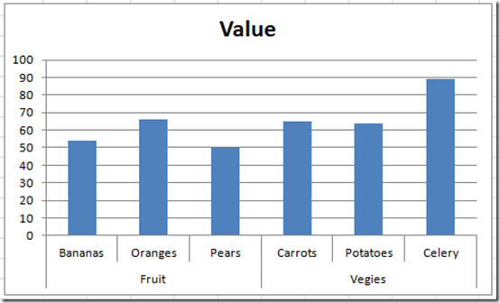
Excel Dashboard Templates Fixing Your Excel Chart When the Multi-Level Category Label Option is ...

DataLabel object (Excel) | Microsoft Docs The following example turns on the data label for the second point in series one on the chart sheet named Chart1, and sets the data label text to Saturday. VB Copy With Charts ("chart1") With .SeriesCollection (1).Points (2) .HasDataLabel = True .DataLabel.Text = "Saturday" End With End With

Excel Column Chart with Primary and Secondary Axes - Peltier Tech Blog

How to Remove Zero Data Labels in Excel Graph (3 Easy Ways) - ExcelDemy Without data labels, column charts may ignore zero data labels, but when we activate the data label option of the chart we can see the zero data labels for the Physics and Maths series also in the chart. To remove this label you can follow this section. Steps: Select the data labels of the Physics series and then Right-click here.

Creating a chart in Excel that ignores #N/A or blank cells - Stack Overflow

How to: Show or Hide the Chart Legend - DevExpress However, to save space in the chart, you can turn this option off by setting the Legend.Overlay property to true. To remove the legend completely, set the Legend.Visible property to false. Worksheet worksheet = workbook.Worksheets ["chartTask3"]; workbook.Worksheets.ActiveWorksheet = worksheet; // Create a chart and specify its location.

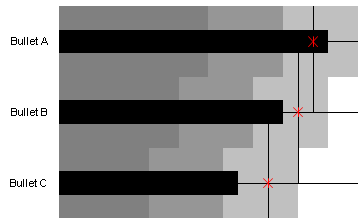
Multiple Horizontal Bullet Graphs in Excel - Peltier Tech Blog

Unable to show gaps for empty cells when plotting chart I am trying to plot a chart that may sometimes contain blank values for the chart area. When I go to change the setting to "show gaps for empty ... Labels: Charting; Charts & Visualizing Data ... In stacked line chart or a 100% stacked line chart you only have zero option. 1 Like . Reply. Larry ONeil . replied to Larry ONeil

Share :